회귀 분석(Regression Analysis)

독립 변수
다른 변수에 영향을 받지 않고 독립적으로 변화하는 수, 설명 변수라고도 함
입력 값이나 원인을 나타내는 변수,y = f(x) 에서 x에 해당하는 것

종속 변수(target)
독립변수의 영향을 받아 값이 변화하는 수, 분석의 대상이 되는 변수
결과물이나 효과를 나타내는 변수, y = f(x) 에서 y에 해당하는 것

잔차(오차항)
계산에 의해 얻어진 이론 값과 실제 관측이나 측정에 의해 얻어진 값의 차이
오차(Error)–모집단, 잔차(Residual)–표본집단

 

 

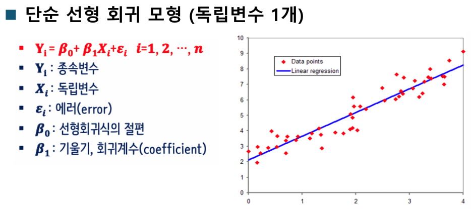
단순 선형 회귀
하나의 특성(Feature, 독립변수)를 가지고 Target을 예측하기 위한 선형 함수를 찾는 것
▪y=ax+b

다중 선형 회귀(Multivariate Linear Regression)
여러 개의 특성을 활용해서 Target을 예측하는 회귀 모델을 만듦
▪y=a[0]x[0]+a[1]x[1]+a[2]x[2]...a[n]x[n]+b

다항 회귀(Polynomial Regression)
입력Feature에 대해 1차 →n차 식으로 변형
데이터가 단순한 직선의 형태가 아닌 비선형 형태인 경우 선형 모델을 사용하여 비선형 데이터를 학습하기 위 한 방법
▪y = a[0]x+a[1]x^2 + b

 

회귀 모형의 4대 가정

선형성

독립변수와 종속변수 간에 선형적인 관계가 있어야 한다.

선형회귀 분석에서 선형성이 만족되지 않으면 모델의 예측력이 떨어질 수 있다
산점도를 통해 확인할 수 있다

원본 데이터도 산점도가 선형성을 보여야 하고 잔차도 중앙값에서 비슷하게 떨어져 있어야한다

위 이미지의 3번 처럼 잔차에서 특징이 발견되면 안된다

# 선형성 확인 

import numpy as np
import matplotlib.pyplot as plt
from sklearn.linear_model import LinearRegression
from sklearn.preprocessing import PolynomialFeatures
from sklearn.pipeline import Pipeline
from sklearn.metrics import r2_score

# 한글
from matplotlib import font_manager, rc
import platform

if platform.system() == "Windows":
    plt.rc("font", family="Malgun Gothic")
elif platform.system() == "Darwin":  # macOS
    plt.rc("font", family="AppleGothic")
else:  # 리눅스 계열 (예: 구글코랩, 우분투)
    plt.rc("font", family="NanumGothic")

plt.rcParams["axes.unicode_minus"] = False  # 마이너스 깨짐 방지

# ----------------------------------------

rng = np.random.default_rng(42)
print(rng)

n = 120


def fit_and_plot_residual(x, y, title, save_prefix=None):
    X = x.reshape(
        -1, 1
    )  # -1은 자동으로 크기를 맞춰라  2차원으로 바꿔야해서. LinearRegression는 2차원만 받음
    model = LinearRegression().fit(X, y)
    y_pred = model.predict(X)
    resid = y - y_pred

    plt.figure(figsize=(6, 4))
    plt.scatter(x, y, alpha=0.7)
    order = np.argsort(x)
    plt.plot(x[order], y_pred[order])
    plt.title(f"y vs X (+Linear Fit) - {title}")
    plt.xlabel("x")
    plt.ylabel("y")
    plt.tight_layout()
    if save_prefix:
        plt.savefig(f"{save_prefix}_scatter_fit.png")
    plt.show()

    plt.figure(figsize=(6, 4))
    plt.scatter(y_pred, resid, alpha=0.7)
    plt.axhline(0, linestyle="--")
    plt.title(f"Residuals VS Fitted - {title}")
    plt.xlabel("Predicted (fitted)")
    plt.ylabel("Resiuals (y-y_pre)")
    plt.tight_layout()
    if save_prefix:
        plt.savefig(f"{save_prefix}_residual.png")
    plt.show()

    return y_pred, resid, model


xA = rng.uniform(-2, 2, size=n)
yA = 2 + 3 * xA + rng.normal(0, 0.8, size=n)
print("xA", xA)

fit_and_plot_residual(xA, yA, "선형성 만족 그래프")

xB = rng.uniform(-2, 2, size=n)
yB = 2 + 3 * xB + 0.7 * (xB**2) + rng.normal(0, 0.8, size=n)
yB_pred, yB_resid, yB_model = fit_and_plot_residual(xB, yB, "부분 위배(선형모델)")
print(f"Case B - Linear model R^2 : ", r2_score(yB, yB_pred))

poly_model = Pipeline(
    steps=[
        ("poly", PolynomialFeatures(degree=2, include_bias=False)),
        ("lin", LinearRegression()),
    ]
)

XB = xB.reshape(-1, 1)
poly_model.fit(XB, yB)
yB_poly_pred = poly_model.predict(XB)
resid_poly = yB - yB_poly_pred

plt.figure(figsize=(6, 4))
plt.scatter(xB, yB, alpha=0.7)
order = np.argsort(xB)
plt.plot(xB[order], yB_poly_pred[order])
plt.title(f"y vs X (+Linear Fit)")
plt.xlabel("x")
plt.ylabel("y")
plt.tight_layout()
plt.show()

plt.figure(figsize=(6, 4))
plt.scatter(yB_poly_pred, resid_poly, alpha=0.7)
plt.axhline(0, linestyle="--")
plt.title(f"Residuals VS Fitted")
plt.xlabel("Predicted (fitted)")
plt.ylabel("Residuals (y-y_pre)")
plt.tight_layout()
plt.show()

 

독립성

독립변수(X) 간에 상관관계가 없어야 한다
다중 선형회귀 분석에서 더욱 중요한데, 독립변수들 간에 높은 상관관계가 있으면 다중공선성(Multicollinearity) 문제가 발생할 수
있다(변수 선택법(Variable Selection)을 사용하여 문제를 해결)
시각화로는 확인하기 어렵다
독립변수간의 독립성을 검증할 때 : VIF로 확인
잔차의 독립성을 검증할 때 : 통계량(Durbin-Watson)으로 확인

 

다중공선성이란.

독립 변수들 사이에 강한 상관관계(선형관계)가 존재하는 상황
계수 추정이 불안정해 짐
훈련 성능은 높으나 실제 성능은 떨어질 확률 높음
진단 방법 : VIF((variance inflation factor)로 진단 5 이상(엄격) 또는 10 이상(관대)면 다중 공선성이 있다고 의심

 

완화 방법
특성 선택/통합
정규화(규제) : Ridge(L2), Lasso(L1), Elastic Net 
차원 축소
더미처리 주의
모델 교체

# 다중공정성 확인 VIF

import numpy as np
import pandas as pd
import statsmodels.api as sm
from statsmodels.stats.outliers_influence import variance_inflation_factor

n = 200
x1 = np.random.normal(size=n)
x2 = 0.9 * x1 + np.random.normal(scale=0.1, size=n)
x3 = np.random.normal(size=n)

df = pd.DataFrame({"x1": x1, "x2": x2, "x3": x3})
print(df.head())


def compute_vif(df_feature: pd.DataFrame) -> pd.DataFrame:
    X = sm.add_constant(df_feature)
    vif_rows = []
    for i in range(X.shape[1]):
        vif_val = variance_inflation_factor(X.values, i)
        vif_rows.append((X.columns[i], vif_val))
    return (
        pd.DataFrame(vif_rows, columns=["features", "VIF"])
        .sort_values("VIF", ascending=False)
        .reset_index(drop=True)
    )


vif_df = compute_vif(df)

print(vif_df)
"""
x1과 x2의 VIF 값이 매우 높음 (보통 10 이상이면 다중공선성 의심)

이는 x1과 x2가 거의 같은 정보를 담고 있어서
회귀 모델에서 계수 추정의 불안정성을 유발할 수 있음을 의미함.

반면 x3는 x1, x2와 독립적이라 VIF ≈ 1 정도로 정상적."""

 

 

# 자기 상관 확인 Durbin-Watson. 전차들이 독립적인지 (자기상관이 있는지) Durbin–Watson 통계량으로 판단
import numpy as np
import pandas as pd
import statsmodels.api as sm
from statsmodels.stats.stattools import durbin_watson
import matplotlib.pyplot as plt

rng = np.random.default_rng(42)
x = np.arange(1, 21)

# y = 3 * x + rng.normal(0, 3, size=20) # 독립 잔차를 더함 0.23
y = 3 * x + np.cumsum(rng.normal(0, 3, size=20))  # 이전까지의 잡음을 누적합함 0.6

X = sm.add_constant(x)
model = sm.OLS(y, X).fit()
resid = model.resid
dw = durbin_watson(resid)
print("Durbin-Watson 통계량: ", dw)

# 0~1 양의 자기 상관 (잔차들이 비슷한 방향으로 움직인다)
# 1~3 독립적(이상적: 2근처)
# 3~4 음의; 자기 상관

 

등분산성

오차(혹은 잔차)의 분산이 독립변수와 무관하게 일정해야 한다.
오차와 독립변수간에 아무런 관련성이 없게 무작위적으로 고루 분포되어야 한다.
등분산성이 만족되지 않으면 이분산성(Heteroscedasticity)이 나타나며, 이는 회귀계수의 표준오차에 영향을 미친다.
등분산성은 잔차 그래프를 통해 확인할 수 있다

 

정규성

잔차가 정규분포를 따라야 한다.
정규성이 크게 위배되면 회귀계수의 유의성 검정에 문제가 생길 수있다
Q-Q 플롯이나 정규성 검정(예: Shapiro-Wilk 검정)을 통해 확인할수 있다 (Q-Q 플롯의 대각선 위로 잔차들이 위치해야 함)

Shapiro-Wilk 검정을 실시 했을 시
• 귀무가설 : 잔차가 정규분포이다,
• 대립가설 : 잔차가 정규분포가 아니다
• P-value > 0.05(유의수준) : 귀무가설을 기각할 수 없다 반대이면 기각

 

실습

# linear_regression() 사용
# horsepower, weight 선형성검증하고 다항식 추가해서 성능 개선
import numpy as np
import pandas as pd
import matplotlib.pyplot as plt
from sklearn.model_selection import train_test_split, KFold, cross_val_score
from sklearn.preprocessing import StandardScaler, PolynomialFeatures
from sklearn.pipeline import Pipeline
from sklearn.linear_model import LinearRegression, RidgeCV
from sklearn.metrics import r2_score, mean_squared_error, mean_absolute_error
import statsmodels.api as sm
from statsmodels.stats.outliers_influence import variance_inflation_factor
import seaborn as sns

# 한글
from matplotlib import font_manager, rc
import platform

if platform.system() == "Windows":
    plt.rc("font", family="Malgun Gothic")
elif platform.system() == "Darwin":  # macOS
    plt.rc("font", family="AppleGothic")
else:  # 리눅스 계열 (예: 구글코랩, 우분투)
    plt.rc("font", family="NanumGothic")

plt.rcParams["axes.unicode_minus"] = False  # 마이너스 깨짐 방지

# ----------------------------------------

df = sns.load_dataset("mpg").dropna().copy()
print(df.info())

X = df[["horsepower", "weight"]]
y = df["mpg"]

x_tr, x_te, y_tr, y_te = train_test_split(X, y, test_size=0.2, random_state=42)

fig, axes = plt.subplots(2, 2, figsize=(10, 8))

# 산점도
sns.regplot(x="horsepower", y="mpg", data=df, ax=axes[0, 0], line_kws={"color": "red"})
sns.regplot(x="weight", y="mpg", data=df, ax=axes[0, 1], line_kws={"color": "red"})
axes[0, 0].set_title("horsepower vs mpg")
axes[0, 1].set_title("weight vs mpg")

# 잔차
sns.residplot(
    x="horsepower",
    y="mpg",
    data=df,
    ax=axes[1, 0],
    lowess=True,
    line_kws={"color": "red"},
)
sns.residplot(
    x="weight", y="mpg", data=df, ax=axes[1, 1], lowess=True, line_kws={"color": "red"}
)
axes[1, 0].set_title("horsepower residuals")
axes[1, 1].set_title("weight residuals")

plt.tight_layout()
plt.show()

# 단순 선형회귀
lin_pipe = Pipeline(
    steps=[("scaler", StandardScaler()), ("lin_model", LinearRegression())]
)
lin_pipe.fit(x_tr, y_tr)
y_pred_lin = lin_pipe.predict(x_te)

r2 = r2_score(y_te, y_pred_lin)
mae = mean_absolute_error(y_te, y_pred_lin)
mse = mean_squared_error(y_te, y_pred_lin)
RMSE = np.sqrt(mse)
print("Linear Regression 성능:")
print("R2 :", r2)
print("mae:", mae)
print("mse :", mse)
print("RMSE :", RMSE)

# 다항식 추가
poly_pipe = Pipeline(
    [
        ("poly", PolynomialFeatures(degree=2, include_bias=False)),
        ("scaler", StandardScaler()),
        ("model", LinearRegression()),
    ]
)
poly_pipe.fit(x_tr, y_tr)
y_pred_poly = poly_pipe.predict(x_te)

print("\nPoly Regression 성능:")
poly_r2 = r2_score(y_te, y_pred_poly)
poly_mae = mean_absolute_error(y_te, y_pred_poly)
poly_mse = mean_squared_error(y_te, y_pred_poly)
poly_RMSE = np.sqrt(poly_mse)
print("R2 :", poly_r2)
print("mae:", poly_mae)
print("mse :", poly_mse)
print("RMSE :", poly_RMSE)

print("\n 변경 값 (poly - line)")
print("R2 :", poly_r2 - r2)
print("mae:", poly_mae - mae)
print("mse :", poly_mse - mse)
print("RMSE :", poly_RMSE - RMSE)

plt.figure(figsize=(6, 4))
plt.scatter(y_te, y_pred_lin, label="Linear", alpha=0.6)
plt.scatter(y_te, y_pred_poly, label="Poly", alpha=0.6)
plt.plot([y_te.min(), y_te.max()], [y_te.min(), y_te.max()], "r--")
plt.xlabel("True mpg")
plt.ylabel("Predicted mpg")
plt.legend()
plt.title("다항식 추가 전 후 비교")
plt.tight_layout()
plt.show()

"""
Linear Regression 성능:
R2 : 0.6514190280854426
mae: 3.5056538974903253
mse : 17.791776112838146
RMSE : 4.218029885247157

Poly Regression 성능:
R2 : 0.6883062442194608
mae: 3.0211866941739345
mse : 15.909031087262887
RMSE : 3.988612677017272

 변경 값 (poly - line)
R2 : 0.03688721613401824  좋아는 졌는데 큰 의미 없음
mae: -0.4844672033163908  0.4만큼 덜 틀림
mse : -1.8827450255752591  
RMSE : -0.2294172082298851  모델 오차가 10%정도 줄음. 유의미한 성능 향상

"""